
— Last updated on March 15, 2024 —
Patch-clamp is still the gold-standard technique to study the intrinsic electrophysiological properties of individual neurons as well as the synaptic communication between neurons. The analysis of the patch-clamp recordings is a crucial step, although it can be challenging for beginners. To help with this, I have written a series of tutorials on patch-clamp data analysis for Python and Clampfit.
In this tutorial, I explain how to analyze postsynaptic currents and potentials using Clampfit, a user-friendly electrophysiological software used in many laboratories. The software is only for Windows, but it seems it can be run on Mac OS as well using CrossOver, WinneBottler or PlayOnMac. The basics of the tutorial should also apply to the analysis in Python (tutorial) or other electrophysiology software. Do not forget, “the best software is the one you know how to use.”
Please contact me if you have suggestions or corrections to improve this tutorial. I hope you find it useful.
Contents
- Introduction
- Example data
- Recording protocol in Clampex
- Data analysis in Clampfit
- Event statistics
- References
Introduction
Synaptic transmission is the electrochemical mechanism that enables the communication between neurons through chemical signals called neurotransmitters, although there are pure electrical synapses too. In general, the action potentials of presynaptic neurons travel along the axon, releasing neurotransmitters into the synaptic gap. Then, neurotransmitters trigger a chemical and electrical signal in the dendrites and cell bodies of postsynaptic (after the synapse) neurons. This pathway is crucial for communication in the nervous system. A kind of “central dogma of neuroscience”, exceptions included.
The high temporal precision of the whole-cell patch-clamp technique can give an informative readout of synaptic transmission by recording postsynaptic currents (ions moving through channels) and potentials (electrical potential differences between the intracellular and the extracellular space). Both currents and potentials can be either excitatory, if they make the neuron more excitable, or inhibitory if they make the neuron less excitable. These postsynaptic electrical responses can increase or decrease over time as a result of synaptic plasticity mechanisms such as short-term plasticity, long-term potentiation, and long-term depression.
Furthermore, it is possible to study the local connectivity of brain areas by patching two (pair recordings) or more neurons (multipatch, see video) simultaneously. Briefly, a set of current pulses are injected into the presynaptic neuron and the postsynaptic potentials or currents are simultaneously recorded in the other patched neurons. The analysis can identify whether the synapses are inhibitory or excitatory, and quantify properties like amplitude, kinetics, and spike-timing-dependent plasticity.
In addition, adeno-associated virus (AAV) vectors and Cre mice (post) can be used to label neuronal subclasses and study their role in the crucial balance between inhibition and excitation in neural circuits. These techniques have enabled the discovery of conserved inhibitory circuits (involving somatostatin and parvalbumin interneurons) from mice to humans.
Multi patch-clamp is a very laborious technique but, fortunately, there are now open-access databases of local connectivity created by collaborative projects. If you are interested, you can explore the database Hippocampome of the circuitry of the mouse hippocampus, and the Allen Institute synaptic dataset of neuronal subclasses of the mouse and human cortex (take a look at the paper by Campagnola et al., 2022).
Example data
For this tutorial, I only focus on how to analyze some basic properties of spontaneous excitatory postsynaptic currents (EPSCs) but the tutorial should work for the analysis of both postsynaptic currents and potentials.
As a data example, I use EPSCs recorded from a somatostatin+ (SST+) interneuron (Tremblay et al., 2016) using whole-cell patch clamp electrophysiology. The neuron was recorded in acute slices containing the mouse prefrontal cortex (post) using potassium gluconate internal solution and ACSF external solution (see protocols). Keep in mind that the voltage measured in current and voltage-clamp does not account for the liquid junction potential (LJP) (see Nat Blair’s post to know more). You can calculate the LJP offline using the Clampex LJP calculator. I used Clampfit 10.7 and Clampfit 11.2 (free version) to analyze the data.
For your own recordings, it is important to establish clear inclusion criteria for analysis. Quality criteria standards in whole-cell patch clamp usually include, among others, the formation of gigaseal (>1 GΩ), stable access resistance <20-25 MΩ, leak current within +/- 100 pA, voltage difference before and after sweeps <2-3 mV. These values will partially depend on the experiment, cell type, and brain sample. As an example, see the methods section of Gouwens et al., 2019.
Recording protocol in Clampex
The most simple Clamplex protocol for continuous recordings of synaptic events is the gap-free mode. This mode can be used in either Current clamp (amount of current injected is controlled) to record postsynaptic potentials (PSPs) or Voltage clamp (membrane voltage is controlled) to record postsynaptic currents (PSCs).
- Acquire > New Protocol.
- Mode/Rate.
- Acquisition Mode: Gap-free.Trial Length. Set the duration of the recording. Trial delay: 0, Runs/trial: 1, Sampling rate: 10 or 20 kHz should be enough in most cases. The theoretical minimum is 2 times the analog bandwidth or the highest event frequency, although 2.5 to 10 times is recommended. I recommend reading the Nyquist-Shannon sampling theorem to understand the rationale behind this (e.g., pClamp guide, p.23 and Axon guide 5th ed, p.199 and 225).
- Inputs. Analog Channel #0: current signal (for postsynaptic currents) or voltage signal (for postsynaptic potentials). Note: the names of the channels depend on how you have configured MultiClamp. See the guide from Molecular Devices.
- Outputs. Analog Channel #0: Voltage (for voltage clamp) or current (for current clamp) command signal.
- You can set other parameters as default.
- Mode/Rate.
- Acquire > Save protocol as. Try to save the protocol with a short and informative name that helps you sort it out afterward.
In “standard” potassium gluconate pipette solution, excitatory postsynaptic currents (EPSCs) are recorded as inward currents (“negative”) at RMP and inhibitory postsynaptic currents (IPSCs) as outward currents (“positive”) at more depolarized voltage. For postsynaptic potentials, excitatory postsynaptic potentials (EPSPs) depolarize the membrane (positive peaks), while inhibitory postsynaptic potentials (IPSPs) keep the membrane potential below the (firing) threshold (generally negative peaks, but not always).
Recording solutions and holding voltage can be adjusted according to the objectives of the experiment and these changes influence the direction of the recorded PSCs. For example, with a high chloride concentration in the pipette solution and a holding voltage of around -70 mV, IPSCs are inward currents (see table below for more examples). The change in driving force and expected ion movements can be estimated beforehand with the Goldman-Hodgkin-Katz equation. In addition, receptor antagonists are used to isolate specific neurotransmitter-mediated currents (e.g., blocking GABAA receptors with picrotoxin).
| Internal solution | Holding potential (mV) | Synaptic events | Signal direction |
| K or Cs-based high Cl– | -70 | IPSCs | Inward |
| Cs-gluconate or -MeSO3 | -70 | EPSCs | Inward |
| Cs-gluconate or -MeSO3 | +10 | IPSCs | Outward |
| K-based low Cl– | -60 | EPSCs | Inward |
| K-based low Cl– | -60 | IPSCs | Outward |
Finally, be also aware that the voltage control of the entire membrane (space clamp) of neurons in brain slices is not possible due to the dendritic tree. Space clamp can be improved by, for example, using Cs in the internal solution. To know more about space clamp problems and artifacts: Armstrong and Gilly (1992), Williams and Mitchell (2008).
Record the protocol
Once you achieve the whole-cell configuration, you need to compensate for the capacitance and series resistance. To know why and how to correct them, read Bill Conelly’s post, MultiClamp manuals (p. 26-36), or a HEKA amplifier manual (p. 70-72). Then, wait 3 to 5 minutes for equilibration between the pipette solution and the cell’s internal environment.
In Clampex, the Cell Membrane Test (Tools > Membrane Test) will allow you to monitor the cell and patch quality (see tutorial). Although the online cell membrane properties are not completely accurate, the properties can indicate the quality and type of cell you are recording. It is good practice to save (Online statistics) or write down the membrane test statistics at the very least at the beginning and the end of your experiment.
The sequence and type of protocols will depend on your experiment. The electrophysiology white paper from the Allen Brain Institute shows an example (p. 5). Use the amplifier software (e.g. Multiclamp 700B, see manual) to set and switch between voltage and current clamp modes as required. Then open the recording protocol (Acquire > Open protocol) in Clampex. Before starting the recording, remember to set the name of your recording (File > Set Data File Names) in a way that facilitates easy location and unique identification (more tips here and on the FAIR website). Finally, click the Record button (F2 or Acquire > Record).
Additional metadata can be added to the recording using the comment section of the recording protocol (see the box above) or the “Comment tag” (Acquire > Comment tag) during the recording. The lattter is useful to indicate when a drug or stimulus is approximately applied. For precise synchronization, it is better to use and record TTL signals.
In Clampex, there is also the option of configuring Sequence keys to set protocols with single keys, linking all of them, and running the entire sequence automatically. It looks like a very cool and useful feature for some experiments but I have barely used it. To learn more, read the pClamp tutorial (p. 84) and watch this video from Molecular Devices.
Data analysis in Clampfit
The analysis of synaptic events is time-consuming and complex, particularly for small synaptic events. Luckily, Clampfit and other software packages (StimFit, Neuromatic, EasyElectrophysiology, or the classic MiniAnalysis) facilitate the detection and analysis of synaptic events. Although I have not yet found a stable and currently supported Python package for synaptic analysis (please send me a message if you know any that I should try), I found that the function FindPeaks (Scipy) can do the job (see post).
General options
- General considerations. Do NOT overwrite the raw data. Save the processed files with another name (File > Save as). Optionally, create first a duplicate of the signal and save only the processed signal with another name. Document and report the changes made to the processed files on paper and/or digital files, and keep your files organized. Acquiring good practices in data management is hard but it really pays off. If you do not know how to start, check these guidelines for data management, data organization in spreadsheets, and file naming conventions.
- Open and save files.
- Open
.txtor.csvfiles. File > Open data. This is a cool feature that allows you to open time series data in Clampfit and analyze the file as if it was a Clampex file. Tab-delimited text files work better for multiple signals. When you open the file, you can indicate the units and signal (e.g. dF/F or a.u. for imaging data) and add a time column if necessary. Read more about how to use the binary file converter. - File > Save as… or Export. To “abf” or “atf” (axon text) files.
- Duplicate the file. Edit > Create Duplicate Signal
- Open
- View > Windows default: Save selected Analysis Window settings as default. This is handy when you have to analyze recordings of the same type.
- Cursors
- To measure voltage/current and time differences. You can bring the cursors with Shift + Left mouse click.
- Lock the cursors to each other. Tools > Cursors > Cursor Properties (or double click on cursor): Lock to partner
- Traces
- Transfer traces. Edit > Transfer traces: Results window (to export data) or Graph window (display traces).
- Average traces. Analyze > Average files. A file will be generated with the average traces from the selected files.
- Select sweeps (traces). View > Select sweeps (or mouse right-click).
- Visualize traces. View > Data display: Sweeps, Continue, Concatenated.
- Filtering
- Analyze > Filter. See the pClamp user guide (p. 173) on how to filter the signal and/or noise.
- Analyze > Power Spectrum. You can leave the default options and check the graph for sources of noise in your recording. Yes, that 50 (Europe) or 60 (US) Hz noise peak (see the fantastic Neurogig posts about electrical noise).
- Results. You can find all numerical results in the corresponding Results window sheet.
- Export the numerical results. Besides directly copying the row and columns, it is better to click on the Results window sheet and File > Save as… >
.atffile. The.atffile can be opened directly by Excel and it keeps the format and the names of the columns. Then, you can save it as.csvor Excel file if you want.
- Export the numerical results. Besides directly copying the row and columns, it is better to click on the Results window sheet and File > Save as… >
- Export the traces. See this post.
- Read more about Clampfit options in the pClamp user guide (Help > PDF Manual).
There are two methods to analyze synaptic events in Clampfit. The threshold search is based on an amplitude threshold, as in the detection of action potentials (post), and the template search is based on a sliding template (event shape) that fits events with different amplitudes (Clements and Bekkers, 1997).
Threshold search
- Analyze > Filter.
- Click on Lowpass and select the type of filter and the cutoff (e.g. Bessel 2000 Hz). Bessel is the most commonly used for time-domain analysis because it introduces a minimal overshoot of the signal. You can also apply a bandpass filter with a Highpass of 1 Hz to remove slow baseline oscillations unless you are interested in analyzing those. Read more about filters in the pClamp guide (p. 173).
- Trace selection: Active signal, All visible traces. Then, click OK.
- Analyze > Adjust > Baseline to subtract either a fixed mean, a fixed value, or adjust manually (recommended if the trace is unstable). Click OK and the baseline will be around 0.
- Analyze > Statistics (optional)
- Baseline region: Full trace
- Search Region: Full trace
- Measurements: Standard deviation (pA).
- Select the region for analysis between cursors 1 and 2.
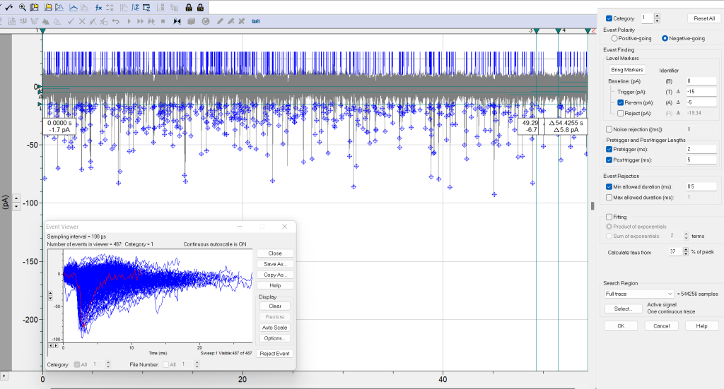
- Event detection > Threshold search (Figure 1, window on the right)
- Category: 1. Note: You can select up to 8 categories with different search criteria, which is useful if there are more than 2 populations of synaptic events.
- Event polarity. Negative-going (for EPSCs in this example).
- Event finding.
- Baseline (pA). Set the baseline at 0 pA (it was adjusted previously).
- Trigger (pA). You can set the threshold level close to the baseline and reject noisy events afterward or use some criteria such as 2.5 or 3 times the standard deviation (calculated before).
- Re-arm (pA). Optional. This value sets the end of the event and the next event is detected when the trigger line is crossed again. Re-arm can be set at the lower bound of the baseline to discard from analysis mini synaptic events that occur during the decay phase of big events. Note that some information will be lost in the analysis.
- Rejection (pA). This can be handy to reject stimulus artifacts (optional).
- Noise rejection (ms). Optional. This can be set to discard from analysis those very short events (e.g., < 1 ms) that cross the trigger.
- Pre-trigger and Post-trigger lengths (ms). To specify the search region before and after the event is detected (when crosses the trigger). For example, pre-trigger: 3 to 5 ms (to set a similar baseline for all events), and post-trigger: between 5 and 15 ms.
- Event rejection. Min and max allowed duration (ms). You can set these values to reject very short or long noisy artifacts.
- Fitting for the rise and decay taus. Three ways. Select either Calculate taus from... (e.g. 37% peak, Chebyshev fitted with a single exponential and no smoothing), Sum of exponentials (as previously but with smooth fitting providing the terms of the fitting, normally 2 for the slow and fast phases), or Product of exponentials (this smooth fitting directly derives the taus from the formula).
- Search region. Cursors 1, 2. Active signal.
- Click OK.
- Click on Accept (event by event), Event detection > Non-stop (fast-forward button), or Event detection > Accept the entire category (next to fast-forward button) to start the section of synaptic events. Events that cross the trigger will be tagged with a diamond symbol at peak amplitude, and two vertical bars delimit the end and start times of the event. See Figure 2.
- Event detection > Event viewer) All current (or voltages) events are displayed here and can be saved (Save as button). See Figure 2. You can also reject individual events.
- Event detection > Define graphs. You can quickly plot different graphs to check, for example, if there is a trend in frequency or amplitude. Choose the type of graph (histogram or scatter plot) and the variables for X and Y (e.g., X: Time of peak, Y: Peak amplitude). You can even select events from these graphs and tag or suppress them in the trace (Event detection > Process selection).
- Event detection > Event statistics. Mean results.
- Results window. Events tab. Results of each synaptic event.
Template search
- Analyze > Filter. E.g. Butterworth (8-pole): 2000 Hz. See pClamp guide (p. 173).
- Analyze > Adjust > Baseline to subtract fixed mean, fixed value, or adjust manually (recommended if the trace is unstable).
- Analyze > Create template
- Zoom in and enclose an event between cursors 1 and 2 and press Add.
- Click on Next and use Align to continue adding events. Fifteen to 20 events might be enough (depending on the variability of the events). The goal is to generate a template representing the “average” time course of the synaptic events in the recording.
- Save the template with Save as.
- Unlock cursors 1 and 2 (lock button) and select the region for analysis between cursors 1 and 2. Note: Select at least 60 seconds to get a representative sample.
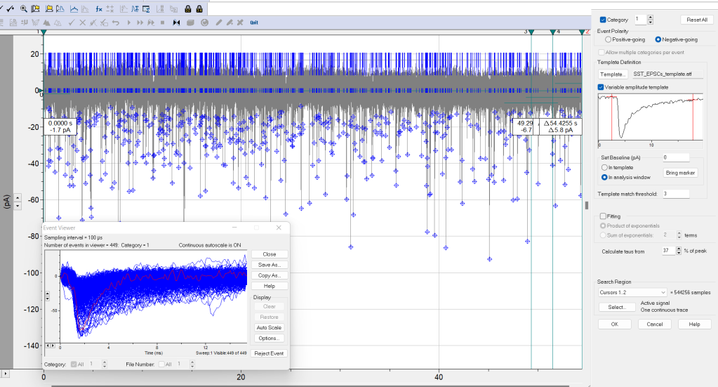
- Event detection > Template search (Figure 2, window on the right).
- Event Polarity: Negative-going (EPSCs in this example) or Positive-going, as required.
- Template. Load template previously saved. Check the option Variable amplitude template. This detects events irrespective of peak amplitude. Move the red vertical cursors to select the template event from baseline pre-event to baseline post-event. Set Baseline (pA). 0 (baseline previously adjusted) or with the red horizontal cursor in the template.Template match threshold: 3 or 4. Note: For most data, 4 times the standard deviation of the noise is optimum (Clements and Bekkers, 1997).
- Fitting for the rise and decay taus. Three ways. Select either Calculate taus from... (e.g. 37% peak, Chebyshev fitted with a single exponential and no smoothing), Sum of exponentials (as previously but with smooth fitting providing the terms of the fitting, normally 2 for the slow and fast phases), or Product of exponentials (this smooth fitting directly derives the taus from the formula).
- Search region: cursors 1 and 2, active signal, continuous trace.
- Click OK.
- Event detection > Save Search Protocol… Save the search parameters as a file (“.spf” extension) that you can name as the recording file and save them together. In this way, you know how you did the analysis and you can always analyze the file with the same parameters: Event Detection > Open Seart Protocol… Note: I do not know the reason, but these handy files do not open in Clampfit 11 (free version). Anyway, always write down the key parameters of your analysis!
- Click on Accept (event by event), Event detection > Non-stop (fast-forward button), or Accept the entire category to count all the synaptic events. Events that cross the trigger will be tagged with a diamond symbol at peak amplitude, and two vertical bars delimit the end and start times of the event. See Figure 2.
- Event detection > Event viewer. All current (or voltages) events are displayed here and can be saved (Save as button). See Figure 2. You can also reject individual events.
- Event detection > Define graphs. You can quickly plot different graphs to check, for example, if there is a trend in frequency or amplitude. Choose the type of graph (histogram or scatter plot) and the variables for X and Y (e.g., X: Time of peak, Y: Peak amplitude). You can even select events from these graphs and tag or suppress them in the trace (Event detection > Process selection).
- Event detection > Event statistics. Mean results.
- Results window. Go to Events tab and you will see the results of each synaptic event.
Event statistics
The results of the synaptic analysis can be tricky to interpret (read Glasgow et al., 2019). As a rule of thumb, postsynaptic potentials are more informative of postsynaptic properties such as synaptic integration and plasticity (Magee, 2000), whereas postsynaptic currents are more related to the presynaptic activity such as neurotransmitter release (Auger and Marty, 2000).
Recording of spontaneous postsynaptic currents (action potentials are not blocked) gives also a good idea of the electrical inputs, mainly in the soma, from the excitatory and inhibitory neurons in the local network. Additionally, it is important to monitor the input resistance (post) because a decrease in input resistance would suggest that more channels are opened, and vice-versa.
To find a definition of the event statistics calculated by Clampfit:
- Go to Help > Clampfit Help.
- In the search bar, type “Event statistics” or navigate to the Menu Reference > Event Detection Menu > Event Statistics section.
- Expand the Peak-time Statistics option to see the definition of each parameter.
Frequency and peak amplitude
In general, the frequency of postsynaptic currents is commonly associated with the presynaptic release of neurotransmitters (probability and the number of release sites), whereas changes in amplitude are a measure of the activation (ionic flux and number) of the postsynaptic receptors. However, a better estimation of these parameters is usually obtained in the absence of presynaptic activity by blocking action with tetrodotoxin (blocks voltage-gated Na+ currents) and miniature postsynaptic currents (mPSCs) are recorded (Turrigiano and Nelson, 2004).
In plasticity experiments, such as long-term potentiation (LTP), it is common to present these and other parameters (e.g., slopes) as a percentage change relative to the baseline (Granger et al., 2013).
Event kinetics
The Event Statistics calculate several parameters of the event kinetics for both the rise and decay phase such as time to rise or decay, rise and decay taus, maximum rise and decay slopes, etc. Time and slopes are calculated by fitting a line to the segment between 10 and 90% of the peak amplitude. The rise time and slope give an idea of how fast the receptors are activated, whereas the decay time and slope measure the rate of receptor deactivation.
When combined with pharmacological or optogenetic (post) experiments, it is possible to study if slower and faster events are modulated by different receptors. For example, the faster kinetics of the synaptic transmission are mediated by AMPA glutamate receptors compared to NMDA glutamate receptors (Watt et al., 2000).
Another interesting parameter is the area (i.e., area under the curve) of the postsynaptic currents (pA · ms), which combines information on the kinetics and the amplitude. The area of the postsynaptic currents is the synaptic charge (Q = I · t), which can give a general estimation of synaptic strength or efficacy. For postsynaptic potentials, the area can be of interest to studying synaptic strength and mechanisms of synaptic integration.
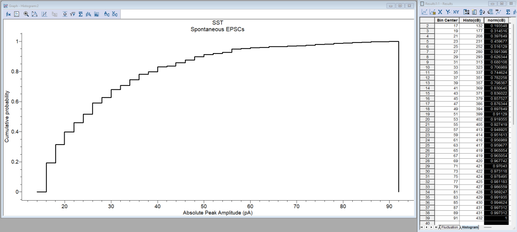
Cumulative histograms and Kolmogorov-Smirnoff test
Cumulative distribution functions (or cumulative histograms) of amplitude (Turrigiano et al., 1998), interevent intervals, and other parameters of synaptic events can be plotted. Then, differences between distributions between, for example, control and drug application, wild-type and transgenic animals, etc., can be tested using the Kolmogorov-Smirnoff test. I prefer to do this analysis in another statistical software package or using R (ggplot2) and Python (post) packages. In any case, you can also do it in Clampfit as follows:
- Results window. Copy the column Peak Amp (pA), Interevent Interval (ms), or other to a new Sheet.
- Results window. Calculate the absolute peak amplitude (optional). Copy the Peak Amplitude column. Analyze > Column Arithmetic. In Expression: cB = cA * (-1), where cA is the column with the peak amplitude values and cB is the new column.
- Analyze > Histogram.
- Distribution: Cumulative.
- Bins. Width. The width will depend on the data (peak amp or interevent interval).
- Data. Select the correct column from the sheet.
- Row Range: Full column.
- Click OK.
- Graph window. The Histogram is created with the count of amplitudes or interevent intervals in each bin.
- Results window. Histogram tab. Optional: Normalize the count values.
- Select the Histo(cA) column, Analyze > Column Arithmetic. In Expression: cC = norm(cB). Note: “c” means column so replace “B” (the column with Histo(cA) data) and “C” (the new column with the normalized data) if needed.
- Analyze > Create Graph.
- Plot type: Histogram.
- Data Type: X-Y pairs.
- Columns in Plot. X >> Bin Center. Y >> “New normalized column”.
- Assign Plots to Graph. Click on Add.
- Click OK to get the graph. See Figure 3.
- Repeat the previous steps if you need to compare two datasets. Select both columns.
- Analyze > Kolmogorov-Smirnoff Test.
- Preprocessing: Ascending sort.
- You can leave the rest of the options as default.
- Click OK.
- Results window. Basic Stats tab. See the K-S statistic (the test D statistics is the maximum difference between the cumulative histograms) and the probability (p-value).
Variance-mean analysis
Just to give a final example of the many possibilities of the analysis of synaptic events, you can estimate parameters of transmitter release from postsynaptic currents recordings using Analyze > V-M Analysis. For this analysis, you need to record the postsynaptic currents under different release probability conditions by changing the external concentration of ions such as the Ca2+/Mg2+ ratio, or Cd2+. Then, the variance (V) and mean (M) of the PSCs are plotted in a V-M graph (Figure 4). The resulting scatter plot is a parabola, in which the slope is related to the quantal amplitude (Q), the curvature is related to the probability of release at each site (P), and the amplitude is related to the number of release sites (N).
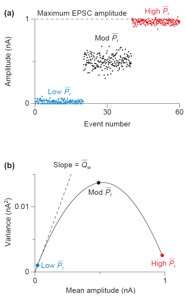
The variance-mean analysis is based on the model of quantal neurotransmitter release, as described in the classic papers by Katz and colleagues. They discovered that neurotransmitters are released from the presynaptic neuron in packages of neurotransmitters known as quanta. Besides, the fusion and release of neurotransmitter vesicles are stochastic processes that follow Poisson or binomial distributions. Although there are many nuances to consider, such as silent synapses, these principles of synaptic transmission remain valid.
To learn more about the analysis, you can read Clements and Silver (2000), Clements (2003), and Silver (2003). Another clear explanation of the variance analysis is provided by Huijstee and Kessels (2020).
References and further reading
- Books
- Aidley, 1998. The Physiology of Excitable Cells. Chapters 7-12.
- Grazina and Dong, 2016. Electrophysiological Analysis of Synaptic Transmission. Protocols and explanations on measuring and analyzing synaptic transmission using patch clamp electrophysiology.
- Johnston and Miao Sin-Wu, 1994. Foundations of Cellular Neurophysiology. Chapters 13-16.
- Clampfit
- Clampfit: Threshold Event Detection Tutorial. Molecular Devices. A longer and more detailed version of the template search analysis.
- Clampfit: Template Event Detection Tutorial. Molecular Devices. Video tutorial (min. 10 to 20). This PDF presentation from Molecular Devices also includes the template search tutorial.
- Papers
- Linders et al., 2022. Studying Synaptic Connectivity and Strength with Optogenetics and Patch-Clamp Electrophysiology. Good review.
- Südhof and Malenka, 2008. Understanding Synapses: Past, Present, and Future. A comprehensive review that covers key discoveries in synaptic physiology, including the role of postsynaptic AMPA receptors in long-term plasticity, and silent synapses.
- More tutorials and resources for patch clamp data analysis.
